OpenTelemetry Collector Sizing

Ask five people how big an OpenTelemetry collector gateway needs to be, and four of them will answer in gigabytes per day. That number tells you almost nothing about whether the box will fall over, because the two resources a collector actually spends — CPU and memory — are driven by two different things, and only one of them is throughput.

TL;DR — CPU scales with throughput: spans, log lines and data points per second. Memory scales with cardinality: the count of distinct active time series held in the pipeline, which has no fixed relationship to how much data is flowing per second. A collector can be nearly idle on CPU and still get OOM-killed on memory, and the usual fix — add more instances — solves the first problem and not the second, because round-robin load balancing still exposes every instance to close to the full series count. What follows is a worked method: real ratios, a full derivation from ratios to VM shapes and instance counts, named reserve factors instead of an implicit buffer, failover math, and a rescale rule with actual thresholds.

This is a small, generalized cost model, not a specific customer’s numbers or a specific vendor’s product: four formulas, four named reserve factors, and the arithmetic to turn a nominal ingest rate into VM shapes, instance counts and load-balancer bandwidth. Adapt it to your own gateway rather than treating any single number here as a constant.

Why the GB/day number keeps failing you

“How many gigabytes a day” is a reasonable question for a log-storage budget. It is close to useless for a collector gateway, because a collector’s memory is not proportional to data volume — it is proportional to how many distinct things it is tracking at once. Ten thousand log lines a second from one well-behaved application is a light memory load. Ten thousand data points a second spread across two hundred thousand distinct label combinations — pod, container, endpoint, a customer ID that leaked into a label — is a heavy one, at the same throughput.

Sizing by GB/day answers the CPU question reasonably well and quietly skips the memory question altogether. That gap is exactly where an under-provisioned gateway gets discovered, at 2am, as an OOM kill.

The two resources that actually matter

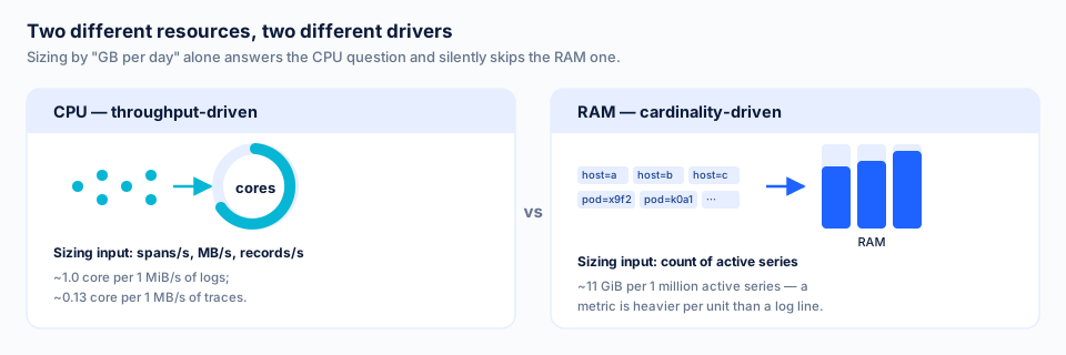
A workable set of ratios for sizing an OTel-based collector gateway, per unit of throughput or cardinality:

• Logs — roughly 1.0 CPU core and 120 MiB of RAM per 1 MiB/s of ingest. CPU-heavy per byte relative to the others, because log processing (parsing, regex, multiline handling) is CPU work.
• Metrics — roughly 0.4 CPU core and 11 GiB of RAM per 1 million active series. RAM-heavy, and the reason is structural: every active series is a live object the pipeline has to track state for, for as long as it stays active, regardless of how often it is scraped.
• Traces — roughly 0.13 CPU core per 1 MB/s of span data; lighter on both axes than the other two signals at comparable volume.

Read across the three, one thing should jump out: metrics carry more than a thousand times the memory cost per unit of “stuff flowing through” that logs do. A workload that is mostly metrics will be memory-bound long before it is CPU-bound, and a sizing exercise that only asks “how many MB/s” will size the CPU correctly and the memory wrong by an order of magnitude.

The trap: horizontal scaling doesn’t fix cardinality

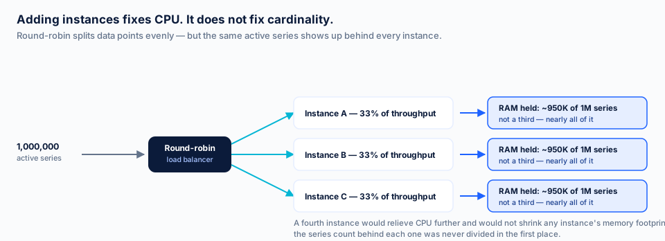
This is the piece that catches people who have read the ratios and sized correctly for a single instance, then hit a wall when they scale out. The instinct is: memory is too high on one box, so put three boxes behind a load balancer and each one carries a third of the load.

That works for CPU. Round-robin distributes individual data points, not whole series — and because the same series recurs on nearly every scrape or every batch, each instance ends up seeing close to the full active-series count, not a fraction of it. Three instances behind a round-robin balancer, each provisioned for “a third of the metrics load,” will each independently approach the memory footprint of the whole workload. A fourth instance relieves CPU further and does nothing for memory, because the cardinality problem was never divided — only the throughput was.

The practical fix is routing traffic so that a given series consistently lands on the same instance (consistent hashing on a stable identity, rather than round-robin), so the series count actually splits across the fleet instead of being replicated across it. That is a different sizing conversation than “how many boxes,” and it is the one worth having before the fleet grows, not after the third OOM kill.

From ratios to instances: a worked sizing model

Turn the per-unit ratios into complete VM shapes with four formulas. Each folds in a named reserve factor rather than a hidden fudge number:

• CPU (cores) = Logs[MiB/s] × 1.0 × 1.5 (DLP overhead) + Traces[MB/s] × 0.13 + Series[millions] × 0.4 + 1 (baseline)
• RAM (GiB) = (Logs[MiB/s] × 0.12 + Traces[MB/s] × 0.17 + Series[millions] × 11 + 2 (baseline)) × 1.25 (memory headroom)
• Load-balancer bandwidth = nominal ingest rate × 8 (MB/s → Mb/s) × 1.5 (burst reserve)
• Queue disk = egress peak × bridge time (a deliberately conservative 90 minutes) × 1.3 (queue reserve)

Apply those across five ingest tiers and you get a small set of shapes to place a workload into, instead of sizing from scratch every time:

Tier	Nominal rate	vCPU / instance	RAM / instance	Queue disk	Instances	LB bandwidth
Default	5 MB/s	8	16 GiB	40 GB	2	60 Mb/s
Small	10 MB/s	16	32 GiB	70 GB	2	120 Mb/s
Medium	20 MB/s	24	64 GiB	140 GB	2	240 Mb/s
Big	30 MB/s	24	64 GiB	210 GB	3	360 Mb/s
Super	50 MB/s	24	128 GiB	350 GB	4	600 Mb/s

A few things worth reading off this table rather than past it:

• The vCPU and RAM values are deliberately round numbers — powers of two you can map onto whatever instance catalog you actually have, not a specific vendor’s SKU list. Treat them as shapes to fit, not as a shopping list.
• Instance count is not simply “more throughput, more boxes.” Big and Super both step up instance count as much as they step up per-instance size, because past a certain size a single instance becomes a larger blast radius on failure — see N+1 below.
• This table sizes CPU and throughput. It does not divide cardinality. A fleet’s active-series count doesn’t shrink because the fleet has more instances — see the trap above. If a workload’s cardinality is unusually high for its throughput, it will out-grow this table’s RAM column before it out-grows the CPU or bandwidth columns, and the fix is consistent-hash routing, not another instance.

Read the formulas as a starting derivation, not a substitute for load-testing your own workload — cardinality especially varies enormously by environment. What the table buys you is a shared vocabulary: “this fleet is roughly a Medium” is a sentence a whole team can use, where “give it about 20 gigs, I think” is not.

Naming your reserve factors

Most sizing conversations have an implicit buffer baked in somewhere — “we’ll round up a bit” — that nobody can point to later. The model above names each one instead, so a number can be audited rather than just trusted:

• DLP overhead (×1.5 on the CPU logs term) — headroom for inline data-loss-prevention processing (masking, redaction) on the log path, which is real CPU work the base ratio doesn’t include.
• Memory headroom (×1.25 on the whole RAM figure) — the gap between the memory limit you set and the memory the workload is actually sized to need, so the memory limiter has room to intervene before the OS OOM-killer does.
• Burst reserve (×1.5 on load-balancer bandwidth) — headroom above steady-state peak for traffic spikes that are normal, not incidents (a deploy storm, an end-of-hour batch job).
• Queue reserve (×1.3 on queue disk) — margin on top of the raw bridge-time calculation, because an outage during a traffic spike is the case that actually happens.

Four named numbers instead of one vague one means that six months later, when the fleet is bigger than planned, someone can ask “which reserve got eaten” instead of re-deriving the whole sizing from nothing.

N+1: what failover actually costs

If the fleet needs to survive one instance going down without dropping data, size for N+1, not N. At n instances handling a workload, losing one means the remaining n − 1 instances each absorb peak ÷ (n − 1) of the total load — not peak ÷ n, which is what a spreadsheet built for the steady state will assume by default. The table’s Instances column already reflects this: Big and Super step up instance count specifically to keep the failover math survivable, not just to add throughput.

The smaller the fleet, the more this bites: at 3 instances, losing one pushes each survivor from a third of peak to a half. At 10, losing one moves each survivor from a tenth to about an eleventh — barely noticeable. N+1 sizing is cheap at scale and expensive exactly where teams are tempted to skip it: on small fleets, where “add 50% capacity for failover” looks like a big number relative to what is already provisioned.

N+1 shares CPU and throughput across the survivors. It does nothing for memory. The active-series count each survivor was already holding under round-robin doesn’t move when one instance goes down, because it was never divided by instance count in the first place — the cardinality warning above applies just as much to the failover case as to the steady state.

Sizing the queue for backend outages

Size a collector’s export queue in time you can absorb, not in an arbitrary item count. The model above uses a deliberately conservative 90-minute bridge time: queue disk = egress peak × 90 minutes × 1.3 (queue reserve). A queue sized against average throughput rather than peak throughput is a queue sized to fail during exactly the conditions that make an outage worse — size it off the peak, then add the reserve on top.

A rescale rulebook, not “let’s keep an eye on it”

The sizing above answers “how big today.” The operational half is knowing when today’s size stops being enough, and that only works with fixed thresholds decided in advance:

• Scale when: sustained memory above target utilization for a defined window (not a single spike), or active series count crossing the next tier up in the table above.
• Scale before, not after, a known event: a large onboarding, a new Kubernetes cluster being enrolled, a Black-Friday-shaped traffic pattern — anything with a known cardinality or throughput jump gets sized ahead of time, not reacted to.
• Alert on the leading indicator, not the failure: memory trending toward the limit is the signal; an OOM kill is the thing the signal exists to prevent, not the trigger to finally look.

Whatever the actual numbers are for a given fleet, writing them down as thresholds — rather than leaving “we’ll notice if it gets bad” as the plan — is what turns sizing from a one-time exercise into an operational practice.

Operational hygiene that matters at this scale

Three habits matter as much as the arithmetic above, and all three follow from the same fact: the resource under real pressure rarely announces itself as “over budget” — it shows up as latency, or as a kill, unless the limits are already decided and tested.

• Don’t set a hard CPU limit. A CPU limit doesn’t fail loudly — it throttles, and throttling reads as tail latency, which is much harder to diagnose back to “under-provisioned” than a clean error would be.
• Set GOMEMLIMIT to roughly 80% of the memory limit. It gives the Go runtime’s garbage collector room to intervene before the OS OOM-killer does — the difference between a controlled slowdown and a hard kill.
• Load-test at 2–3× the expected peak before anything ships to production. The formulas above are a starting derivation; the load test is what confirms the reserve factors are large enough for a specific workload’s actual burstiness.

Where LinkMesh fits

None of the method above needs a specific product — it is math and measured ratios, and it works whether you run one collector by hand or a thousand through a fleet manager. Where a central control plane earns its place is after the sizing decision: once you know a fleet is going to be, say, a Medium-tier deployment behind consistent-hash routing, LinkMesh pushes that configuration to every instance from one place, and its fleet health view shows you the real per-instance CPU, memory and throughput this article told you to watch — which is what tells you the N+1 reserve is actually being eaten into, instead of finding out from an incident.

If you’re already running a collector fleet you sized by feel, the fastest way to find out whether it’s a tier too small is to look at what it’s actually holding: see LinkMesh’s fleet view on your own collectors and check real numbers against the table above, rather than against a GB/day guess.

For the fleet-management side of this — pushing that sizing decision out consistently once you’ve made it — see how the config-out half of the job compares in Bindplane vs LinkMesh: Where Your Control Plane Runs. For the cost side of the same numbers, How to Reduce Observability Costs covers filtering and sampling to shrink what you have to size for in the first place.

---

Sources: Estimating collector resource usage and Scaling a central telemetry gateway: capacity planning, load testing and production lessons — the per-unit CPU/RAM ratios and operational practices above are adapted from published research on a widely-deployed OTel-compatible collector; the tier table, formulas and reserve factors are this piece’s own derivation.